R stores data in objects that can be inspected, subsetted, and visualized
Load a dataset with read.delim()
Data types (numeric, character, factor, data.frame)
The same object can be explored in different ways
Inspect data structure with str() and summary()
Basic functions: head(), str(), summary()
Factors represent categorical variables used in statistical analysis
Create basic visualizations with ggplot2
R packages and how to load them (library())
Different data types require different visualization approaches
Subset data using $, [ ], and dplyr::filter()
1.2 Getting to Know RStudio
RStudio is an Integrated Development Environment (IDE) for R. When you open RStudio, you will see four panels:
Panel
Location
Function
Console
Bottom left
Where R executes code and displays output
Source Editor
Top left
Where you write and save scripts (.R files)
Environment
Top right
Shows objects in R memory
Files/Plots/Packages/Help
Bottom right
Tabs for file navigation, viewing plots, managing packages, and documentation
Think-aloud (I Do): “I open RStudio and see four panels. The panels I use most often are the Console for running code and the Source Editor for writing longer scripts. When I run code in the Console, the objects I create appear in the Environment panel.”
1.3 Objects and Assignment
In R, we store data in objects using the assignment operator <-:
# Create an object named 'x' containing the number 5x <-5# Create an object named 'name' containing textname <-"BISB211203"# Create an object named 'numbers' containing a sequencenumbers <-c(1, 2, 3, 4, 5)# View the contents of objectsx
[1] 5
name
[1] "BISB211203"
numbers
[1] 1 2 3 4 5
Why <- instead of =? Both can be used, but <- is the R convention. This makes code easier to read and consistent with code written by the R community.
Self-explanation prompts:
1. Why do we need to store data in objects? What’s the difference between typing 5 + 3 directly vs x <- 5; x + 3?
2. What happens if we run x <- 10 after previously setting x <- 5?
1.4 Basic Data Types
R has several data types that are important to know:
Why are factors important? In statistics, factors are used for categorical variables (species type, treatment, soil type). R treats factors differently from character — factors have levels (category levels) that are used in analysis.
1.5 Loading and Inspecting Data
1.5.1 Reading Files
# Read a TSV fileiris_data <-read.delim("assets/data/iris_dataset.tsv")
  sepal.length    sepal.width     petal.length    petal.width
 Min.   :4.300   Min.   :2.000   Min.   :1.000   Min.   :0.100
 1st Qu.:5.100   1st Qu.:2.800   1st Qu.:1.600   1st Qu.:0.300
 Median :5.800   Median :3.000   Median :4.350   Median :1.300
 Mean   :5.843   Mean   :3.054   Mean   :3.759   Mean   :1.199
 3rd Qu.:6.400   3rd Qu.:3.300   3rd Qu.:5.100   3rd Qu.:1.800
 Max.   :7.900   Max.   :4.400   Max.   :6.900   Max.   :2.500
       class
 Length   :150
 N.unique :  3
 N.blank  :  0
 Min.nchar: 11
 Max.nchar: 15
Think-aloud (I Do): “I run str(iris_data) and see that this data has 150 observations and 5 variables. The ‘sepal length’ variable is numeric (numbers), and ‘class’ is a factor (categories). This is important because I will use different data types for different analyses.”
1.5.3Hinge Question
Before continuing, try answering: You run str(student_data) and see the output: Factor w/ 3 levels "A","B","C": 1 1 2 3 2 1. What does “Factor w/ 3 levels” mean?
The data has 3 rows
This column contains 3 categories (categorical variable)
There are 3 columns in the dataset
The values are sorted 1, 2, 3
Answer: B. This is a categorical variable with 3 category levels.
1.6 Data Subsetting
Subsetting means taking a portion of data from a dataset:
# Extract a specific column using $iris_data$`sepal.length`
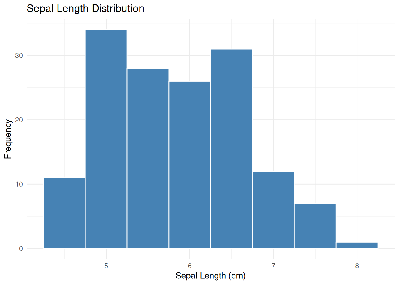
ggplot(iris_data, aes(x =`sepal.length`)) +geom_histogram(binwidth =0.5, fill ="steelblue", color ="white") +labs(title ="Sepal Length Distribution",x ="Sepal Length (cm)",y ="Frequency") +theme_minimal()
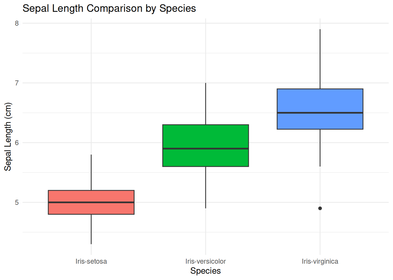
1.7.3 Boxplot
ggplot(iris_data, aes(x =`class`, y =`sepal.length`, fill =`class`)) +geom_boxplot() +labs(title ="Sepal Length Comparison by Species",x ="Species",y ="Sepal Length (cm)") +theme_minimal() +theme(legend.position ="none")
Think-aloud (I Do): “In ggplot2, I always start with ggplot(data, aes(...)) which specifies the data and aesthetic mapping (x and y). Then I add layers with geom_* — geom_histogram() for distributions, geom_boxplot() for group comparisons. labs() adds titles and labels, theme_minimal() gives a clean appearance.”
1.8 Exercises (You Do)
Now it’s your turn! Follow these steps independently:
Try creating different visualizations from the iris dataset:
- Histogram for petal width
- Boxplot of petal length by species
- Scatter plot of sepal length vs sepal width colored by species
1.9 Summary
In this session, we have learned:
- The four RStudio panels and their functions
- Objects and assignment with <-
- Basic data types: numeric, character, factor, logical
- Reading data with read.delim()
- Inspecting data with str(), summary(), head()
- Subsetting data with $, [ ], and dplyr::filter()
- Basic visualization with ggplot2: histograms and boxplots
In the next session, we will use these skills to perform more in-depth statistical analysis — starting with the T-test.