library(ggplot2)
library(dplyr)
Attaching package: 'dplyr'The following objects are masked from 'package:stats':
filter, lagThe following objects are masked from 'package:base':
intersect, setdiff, setequal, unionComparing Means of Two Groups
After this session, students will be able to:
| Know | Understand | Do |
|---|---|---|
| T-test assumptions (normality, homogeneity of variance) | T-test measures how many standard errors separate two means | Perform independent t-test with t.test() |
| Interpretation of t-value, p-value, and Cohen’s d | p-value is the probability of seeing such a difference by chance | Calculate descriptive statistics per group |
| Difference between one-sample, paired, and independent t-tests | Effect size (Cohen’s d) provides practical context beyond statistical significance | Visualize t-test results with ggplot2 |
| Interpretation of t-test results in biological context |
R has the Student’s t-distribution, which is similar to the normal distribution but has heavier tails, especially with small degrees of freedom (df).
library(ggplot2)
library(dplyr)
Attaching package: 'dplyr'The following objects are masked from 'package:stats':
filter, lagThe following objects are masked from 'package:base':
intersect, setdiff, setequal, union# Generate a vector of 100 values between -4 and 4
n <- 100
x <- seq(-4, 4, length = n)
# Create a data frame for ggplot2
df_raw <- data.frame(Index = 1:n, Value = x)
# Plot using ggplot2
ggplot(df_raw, aes(x = Index, y = Value)) +
geom_point(color = "blue") +
labs(
title = "Scatter Plot of Values from -4 to 4",
x = "Index",
y = "Value"
) +
theme_minimal()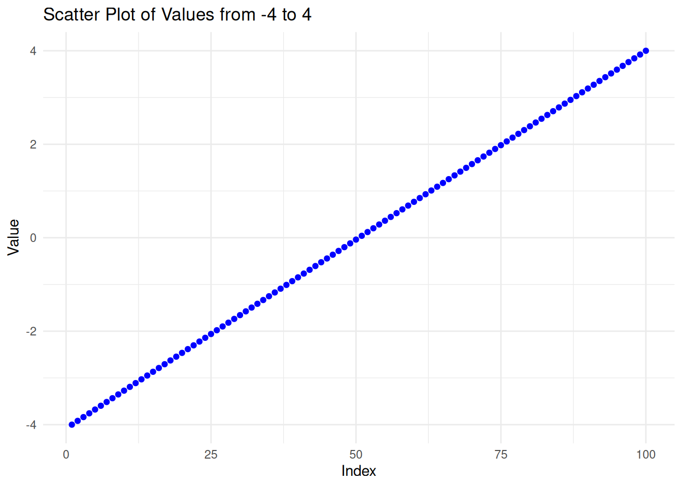
To find the value of the probability density function (pdf) of the Student’s t-distribution given a random variable x, use the dt() function in R.
# Simulate the t-distribution
y <- dt(x, df = n - 1)

# Create a data frame for ggplot2
df_T <- data.frame(Index = 1:n, Value = y)

# Create the scatter plot
ggplot(df_T, aes(x = Index, y = Value)) +
  geom_line(color = "blue") +
  labs(
    title = "T-Distribution",
    x = "Index",
    y = "Value"
  ) +
  theme_minimal()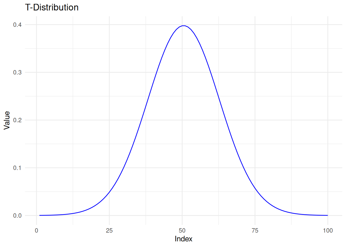
# Step 1: Sample from t-distribution
set.seed(123)
sample_size <- 30
sample_data <- rt(sample_size, df = n - 1)
sample_mean <- mean(sample_data)

# Step 2: Plot with rug (horizontal tick marks showing sample values)
tplot <- ggplot(df_T, aes(x = x, y = y)) +
  geom_line(color = "blue", size = 1.2) +
  geom_vline(xintercept = sample_mean, color = "red", linetype = "dashed", size = 1) +
  geom_rug(data = data.frame(x = sample_data), aes(x = x), inherit.aes = FALSE, sides = "b", color = "black", alpha = 0.5) +
  annotate("text", x = sample_mean, y = max(y) * 0.9,
           label = paste0("Mean = ", round(sample_mean, 2)), color = "red", hjust = -0.1) +
  labs(title = "T-Distribution with Sample Mean",
       x = "t-value", y = "Density") +
  theme_minimal()
Warning: Using `size` aesthetic for lines was deprecated in ggplot2 3.4.0.
ℹ Please use `linewidth` instead.tplot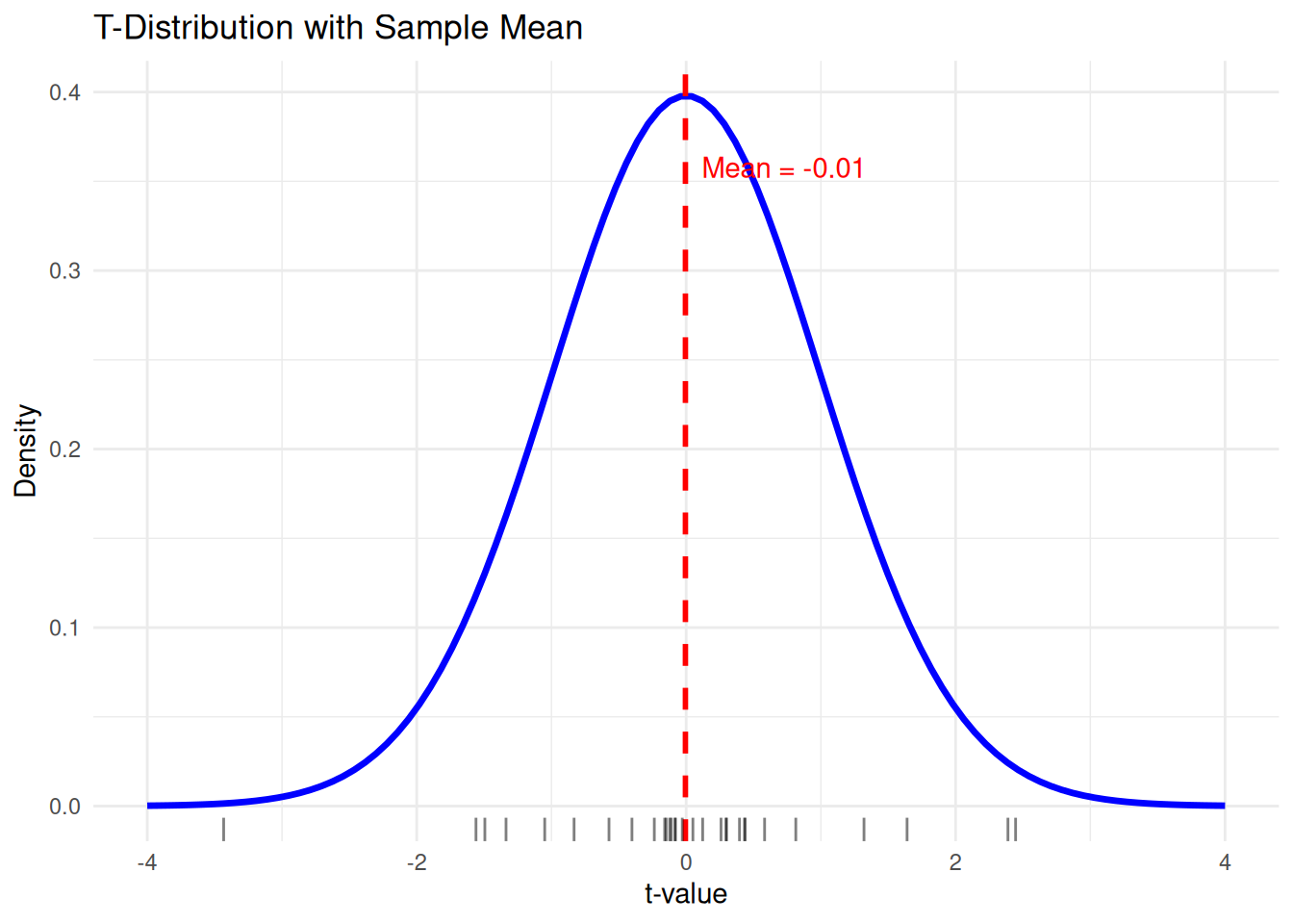
# Step 1: Generate multiple samples
set.seed(123)
sample_size <- 30
n_repeats <- 5

# Store all sample data with sample ID
samples <- lapply(1:n_repeats, function(i) {
  data.frame(Sample = paste0("Sample ", i),
             Value = rt(sample_size, df = n - 1))
}) %>% bind_rows()

# Compute means for each sample
sample_means <- samples %>%
  group_by(Sample) %>%
  summarise(mean = mean(Value))

# Step 2: Base plot with t-distribution
p <- ggplot(df_T, aes(x = x, y = y)) +
  geom_line(color = "blue", size = 1.2) +
  labs(title = "T-Distribution with Multiple Sample Rugs and Means",
       x = "t-value", y = "Density") +
  theme_minimal()

# Step 3: Add rugs and means
# We'll loop through each sample group and add them
for (i in seq_len(n_repeats)) {
  sample_name <- paste0("Sample ", i)
  sample_vals <- samples %>% filter(Sample == sample_name)
  sample_mean <- sample_means %>% filter(Sample == sample_name) %>% pull(mean)

  # Add rug and mean line
  p <- p +
    geom_rug(data = sample_vals, aes(x = Value), inherit.aes = FALSE,
             sides = "b", alpha = 0.4, color = scales::hue_pal()(n_repeats)[i]) +
    geom_vline(xintercept = sample_mean, color = scales::hue_pal()(n_repeats)[i],
               linetype = "dashed", size = 0.8)
}

# Print the plot
p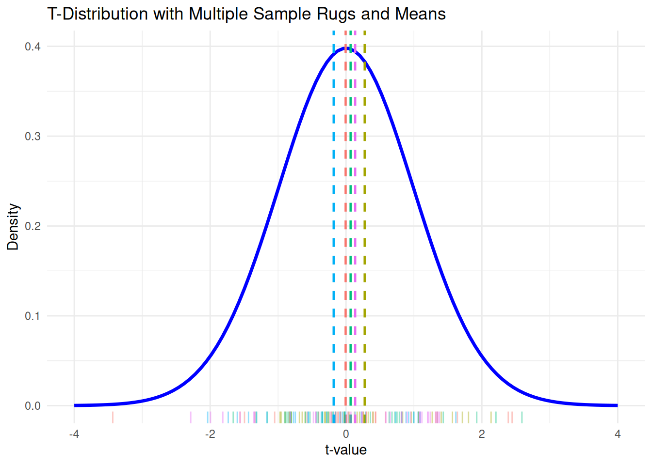
Why is the t-distribution important? The larger the degrees of freedom, the closer the t-distribution is to the normal distribution. In practice, when sample size > 30, the t-distribution and normal distribution are nearly identical.
# Create a data frame with all distributions
df <- data.frame(
  x = rep(x, times = 4),
  density = c(
    dt(x, df = 2),
    dt(x, df = 8),
    dt(x, df = 32),
    dnorm(x)
  ),
  distribution = factor(rep(c("df = 2", "df = 8", "df = 32", "Normal"), each = length(x)))
)

# Plot
ggplot(df, aes(x = x, y = density, color = distribution)) +
  geom_line(linewidth = 1.2) +
  labs(
    title = "Comparison of t-Distributions",
    x = "T Value",
    y = "Density",
    color = "Distribution"
  ) +
  theme_minimal()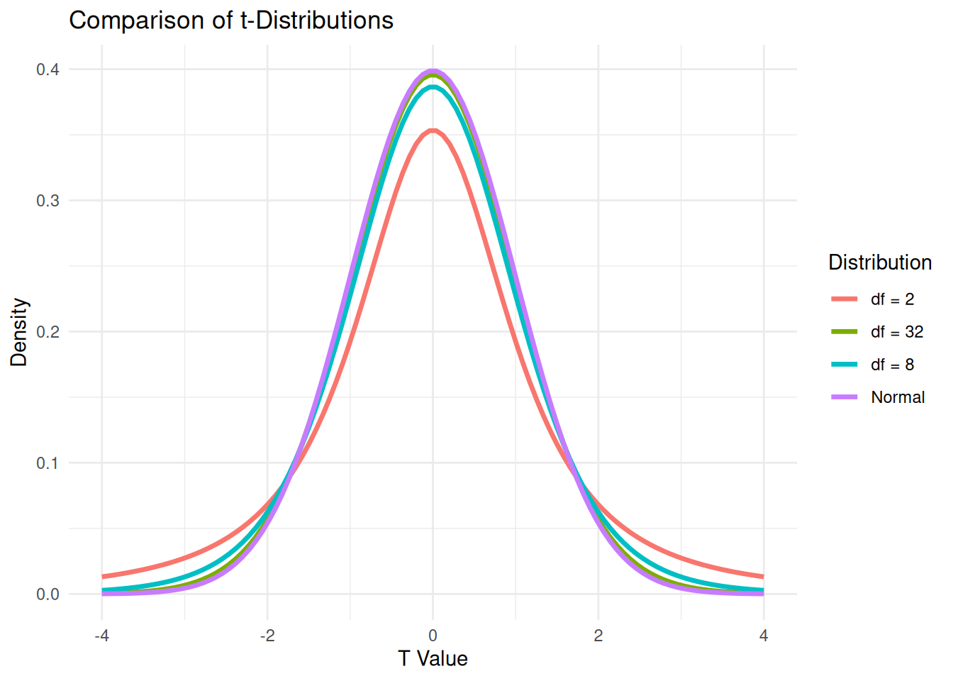
flowchart LR
    Hulu["🏞️ Upstream Lake"] --> Pabrik["🏭 Factory"] --> Hilir["🏞️ Downstream Lake"]

    style Hulu fill:#e1f5fe
    style Pabrik fill:#fff3e0
    style Hilir fill:#ffebee
flowchart LR
Hulu["🏞️ Upstream Lake"] --> Pabrik["🏭 Factory"] --> Hilir["🏞️ Downstream Lake"]
style Hulu fill:#e1f5fe
style Pabrik fill:#fff3e0
style Hilir fill:#ffebee
A group of environmental biologists is conducting a study on the possible ecological impact of a local manufacturing plant. The factory is located between two small lakes that are part of the same river system:
To assess the potential impact, the team collected samples of fish from both lakes. For each fish, they recorded:
The scientists want to determine whether the fish population in the Downstream lake shows any significant difference in size compared to the Upstream lake. Differences in fish size (length or weight) could be an indicator of environmental stress, food availability, or contamination.
Think-aloud (I Do): “I have data from two independent groups — fish from the upstream lake and the downstream lake. I want to compare the mean fish length between the two lakes. An independent t-test is the right choice because I’m comparing two different groups.”
Retrieval Practice: Before continuing, try to recall: - What does
read.csv()do inR? - How do you inspect data structure? - Write the code!
# Import Dataset
fish_data <- read.csv("assets/data/fish_data_weight.csv")

# Quick look
head(fish_data)
Lake Length_cm Weight_g
1 Upstream 26.3 318.7
2 Upstream 27.3 347.7
3 Upstream 32.7 332.6
4 Upstream 28.2 329.6
5 Upstream 28.4 311.5
6 Upstream 33.1 338.6length_stats <- fish_data %>%
group_by(Lake) %>%
summarise(
mean = mean(Length_cm),
sd = sd(Length_cm),
n = n(),
se = sd / sqrt(n),
df = n - 1
)
length_stats# A tibble: 2 × 6
Lake mean sd n se df
<chr> <dbl> <dbl> <int> <dbl> <dbl>
1 Downstream 28.4 2.72 50 0.385 49
2 Upstream 28.1 2.78 50 0.394 49# EXERCISE: CALCULATE DESCRIPTIVE STATISTICS FOR FISH WEIGHT!
# Hint: Follow the pattern from the code above, replace Length_cm with Weight_g# Visualize using scatter plot to see the distribution
ggplot(fish_data, aes(x = Length_cm, y = Weight_g, color = Lake)) +
geom_point(size = 3, alpha = 0.7) +
labs(
title = "Fish Length vs. Weight",
x = "Length (cm)",
y = "Weight (g)",
color = "Lake"
) +
theme_minimal()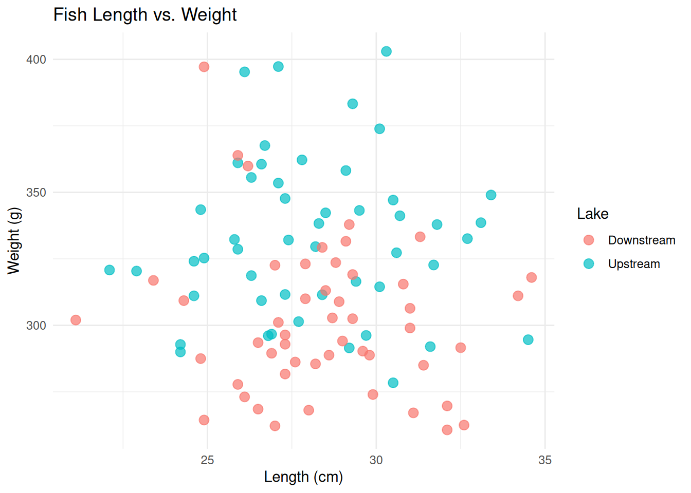
ggplot(fish_data, aes(x = Length_cm)) +
  geom_histogram(position = "identity", alpha = 0.6, bins = 15) +
  labs(title = "Distribution of Fish Length",
       x = "Length (cm)",
       y = "Count") +
  theme_minimal()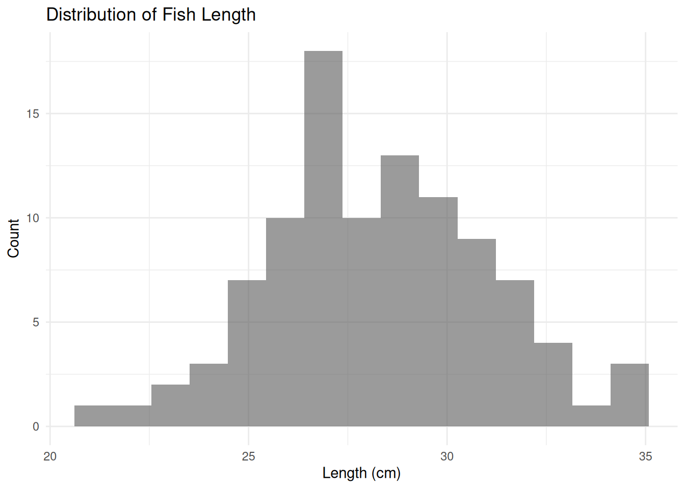
ggplot(fish_data, aes(x = Length_cm, fill = Lake)) +
  geom_histogram(position = "identity", alpha = 0.6, bins = 15) +
  labs(title = "Distribution of Fish Length",
       x = "Length (cm)",
       y = "Count") +
  theme_minimal()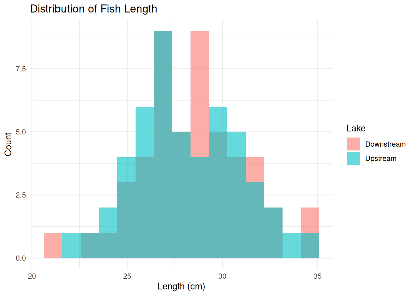
# EXERCISE: PLOT THE DISTRIBUTION OF FISH WEIGHT
# Hint 1: Use geom_histogram() as above
# Hint 2: Replace Length_cm with Weight_g
# Hint 3: Don't forget to change the x-axis label
# Summarise data to get mean and standard error per group
weight_summary <- fish_data %>%
group_by(Lake) %>%
summarise(
mean_weight = mean(Length_cm),
se_weight = sd(Length_cm) / sqrt(n())
)
# Bar plot with error bars
ggplot(weight_summary, aes(x = Lake, y = mean_weight, fill = Lake)) +
geom_col(width = 0.6) +
geom_errorbar(aes(ymin = mean_weight - se_weight,
ymax = mean_weight + se_weight),
width = 0.2) +
labs(title = "Mean Fish Length by Lake",
x = "Lake Type",
y = "Length (cm)") +
theme_minimal()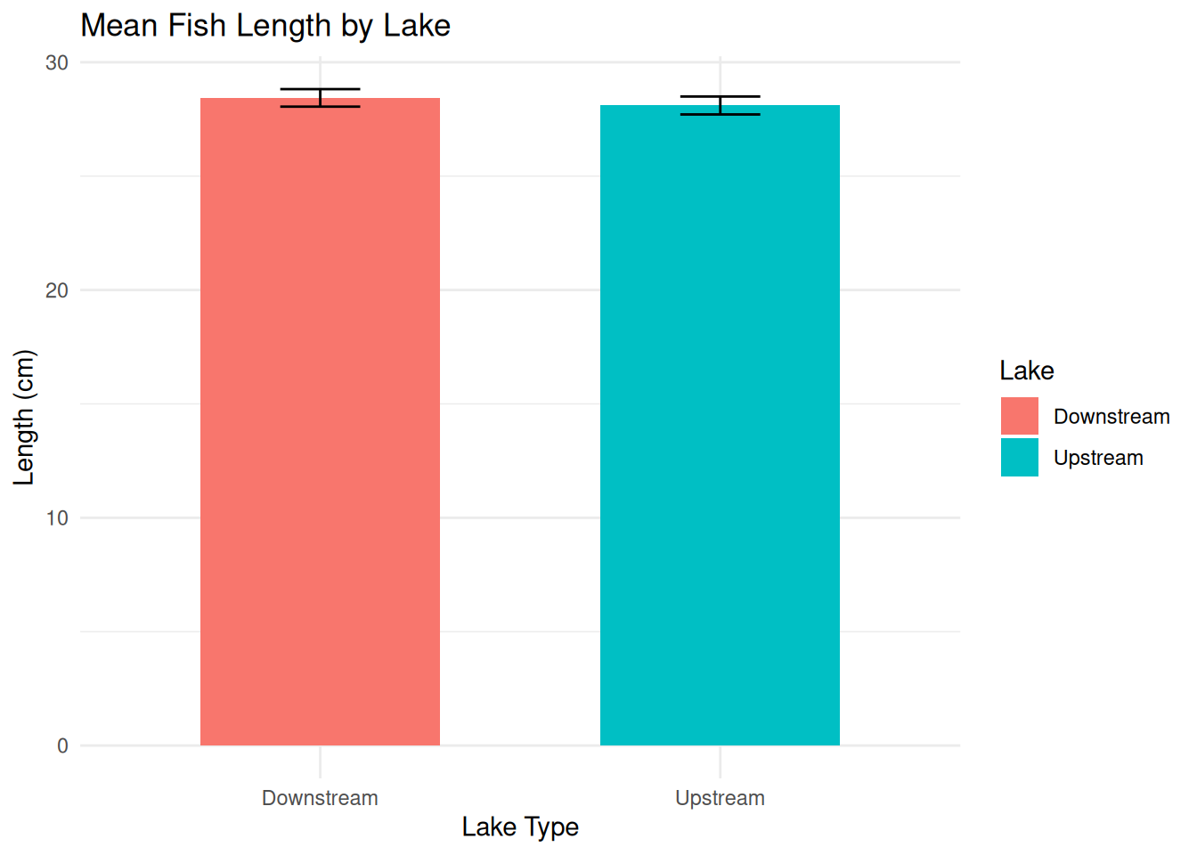
ggplot(fish_data, aes(x = Lake, y = Length_cm, fill = Lake)) +
  geom_boxplot() +
  labs(title = "Fish Length by Lake",
       x = "Lake Type",
       y = "Length (cm)") +
  theme_minimal()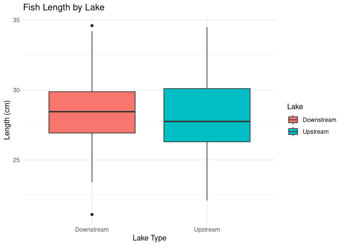
# EXERCISE: CREATE A BARPLOT OF FISH WEIGHT
# Summarise data to get mean and standard error per group
# Hint 1: Use the weight_summary code above as a template
# Hint 2: Replace Length_cm with Weight_g
# Hint 3: Use geom_col() for barplot and geom_errorbar() for error bars

# Bar plot with error bars
# EXERCISE: PLOT THE BOXPLOT FOR FISH WEIGHT
# Hint: Use geom_boxplot() as above, replace Length_cm with Weight_gBefore continuing, try answering: You run a t-test and get this output:
t = 2.45, df = 98, p = 0.016. What is your conclusion?
- No significant difference because p > 0.01
- Significant difference because p < 0.05
- Sample size is too small to make a conclusion
- You need to run ANOVA, not a t-test
Answer: B. Since p = 0.016 < 0.05, we reject the null hypothesis and conclude there is a significant difference.
What you’re testing: > Whether the mean fish length in the Upstream area is significantly different from the Downstream area.
We will calculate the t-statistic → the number of standard errors the means are apart.
Larger t_value → stronger evidence of difference.
The p value gives the probability of seeing such a difference by chance. > - p < 0.05 → statistically significant difference > - p ≥ 0.05 → not statistically significant
Cohen’s d tells you how big the difference is:
| d | Interpretation |
|---|---|
| 0.2 | Small effect |
| 0.5 | Medium effect |
| 0.8+ | Large effect |
Even if p < 0.05, a small Cohen’s d might mean the difference isn’t practically meaningful.
### Perform an Independent t-test (Manual)

# Create subsets
fish_upstream <- subset(fish_data, Lake == "Upstream")
fish_downstream <- subset(fish_data, Lake == "Downstream")

# Means
mean_up <- mean(fish_upstream$Length_cm)
mean_down <- mean(fish_downstream$Length_cm)
mean_diff <- mean_up - mean_down

# Sample sizes
n_up <- nrow(fish_upstream)
n_down <- nrow(fish_downstream)

# Degrees of freedom
df <- n_up + n_down - 2

# Variances
var_up <- var(fish_upstream$Length_cm)
var_down <- var(fish_downstream$Length_cm)

# Pooled standard error
se_pooled <- sqrt((var_up / n_up) + (var_down / n_down))

### t-test Results

# t-value
t_value <- mean_diff / se_pooled

# Two-tailed p-value
p_value <- 2 * (1 - pt(abs(t_value), df = df))

# Cohen's d (effect size)
sd_up <- sd(fish_upstream$Length_cm)
sd_down <- sd(fish_downstream$Length_cm)
pooled_sd <- (sd_up + sd_down) / 2
cohens_d <- mean_diff / pooled_sd

### Print Results
t_value     # how far apart the means are in SE units
[1] -0.6068471p_value # is it statistically significant?[1] 0.5453558cohens_d # how big is the effect?[1] -0.1213778# Use your computed t_value and df
# For example:
# t_value <- 5.87
# df <- 98
alpha <- 0.05
t_crit <- qt(1 - alpha / 2, df = df) # two-tailed
x_vals <- seq(-4, 4, length.out = 300)
y_vals <- dt(x_vals, df = df)
ggplot(data.frame(x = x_vals, y = y_vals), aes(x, y)) +
geom_line(color = "steelblue", size = 1) +
# Shade critical regions
geom_area(data = subset(data.frame(x = x_vals, y = y_vals), x <= -t_crit),
aes(x = x, y = y), fill = "red", alpha = 0.3) +
geom_area(data = subset(data.frame(x = x_vals, y = y_vals), x >= t_crit),
aes(x = x, y = y), fill = "red", alpha = 0.3) +
# Observed t-value
geom_vline(xintercept = t_value, color = "darkgreen", linetype = "dashed", size = 1) +
# Labels
labs(
title = "t-Distribution Under H0",
subtitle = paste0("t-value = ", round(t_value, 2),
", df = ", df,
", alpha = 0.05"),
x = "t-statistic",
y = "Density"
) +
theme_minimal()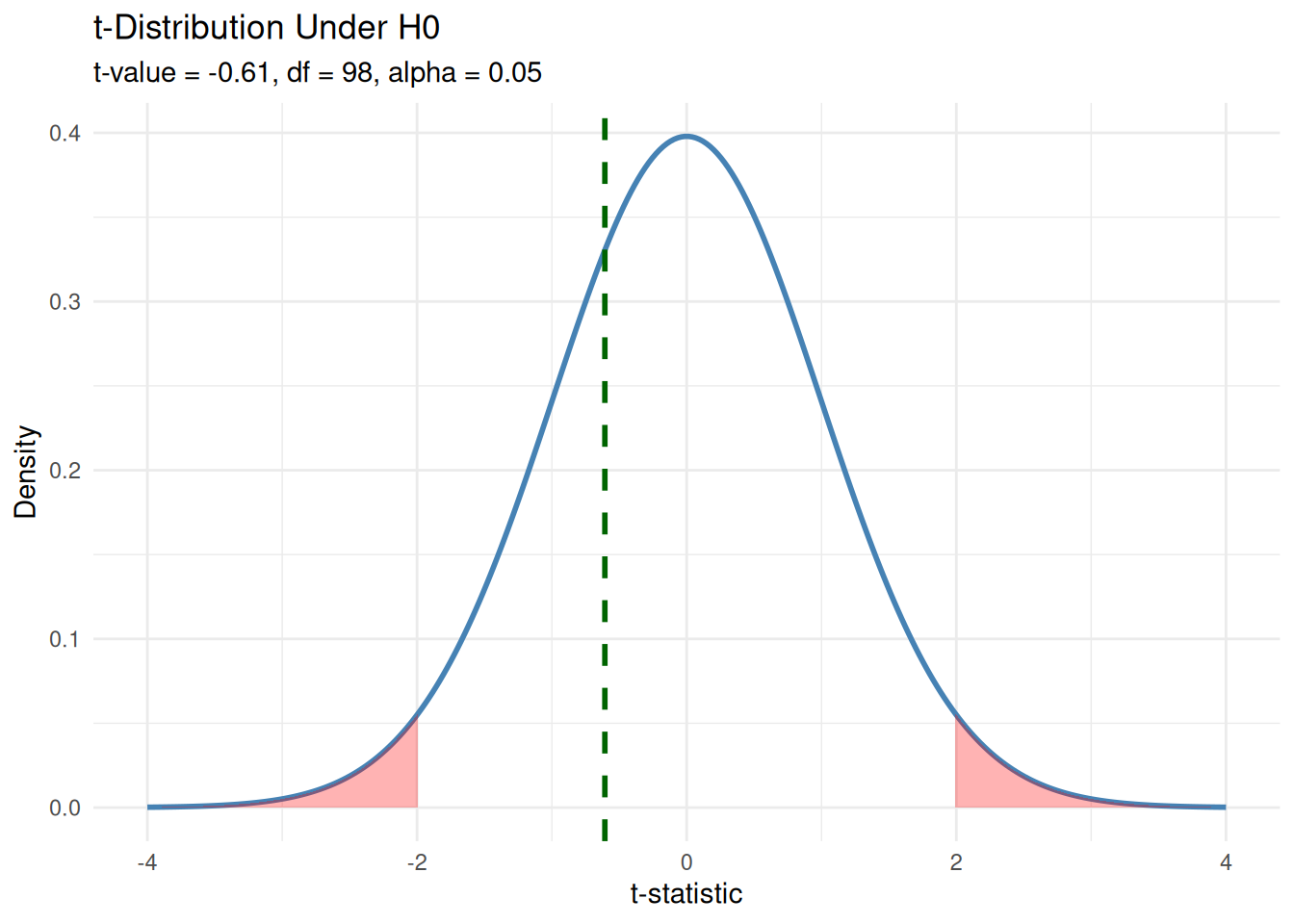
### Independent t-test, the easy way

# Conduct an independent t-test
t_result <- t.test(fish_upstream$Length_cm, fish_downstream$Length_cm, var.equal = TRUE)
t_result
    Two Sample t-test

data:  fish_upstream$Length_cm and fish_downstream$Length_cm
t = -0.60685, df = 98, p-value = 0.5454
alternative hypothesis: true difference in means is not equal to 0
95 percent confidence interval:
 -1.4262226  0.7582226
sample estimates:
mean of x mean of y
   28.102    28.436
# Extract t-value and degrees of freedom
t_value <- t_result$statistic # this is named "t"
df <- t_result$parameter # this is named "df"Using the example above, determine whether there are differences in fish weight between the two populations!
Retrieval Practice: Before working on this, recall: - What function is used to perform a t-test in
R? - How do you split data by group? - Write down the t-test formula shown above!
Hint Ladder: - Hint 1: Use
subset()to split Upstream and Downstream data byWeight_g- Hint 2: Uset.test()with parametervar.equal = TRUE- Hint 3: See the t-test code forLength_cmabove as a reference
### Independent t-test, the easy way

# Run t-test and store the result
# Hint: Replace Length_cm with Weight_g everywhere
fish_upstream_weight <- subset(fish_data, Lake == "Upstream")
fish_downstream_weight <- subset(fish_data, Lake == "Downstream")

# Extract t-value and degrees of freedom
t_result_weight <- t.test(fish_upstream_weight$Weight_g, fish_downstream_weight$Weight_g, var.equal = TRUE)
t_result_weight
# Visualize your t-test result
# Hint: Use the t-test visualization code for Length_cm as a template
# Replace all Length_cm references with Weight_g
# Replace t_value and df with results from t_result_weight